PCR プライマー設計のデファクトスタンダードである primer3。長年 C 言語の本体と、その上に載る Python バインディング primer3-py が定番でしたが、最近になって Rust バインディング primer3-rs が公開されました。
この記事では、「まず動かす」ところを目標に、C 本体・primer3-py と対比しながら primer3-rs の使い方を簡単に紹介します。
primer3 の「3 つのレイヤー」
primer3 まわりのツールは、同じ C エンジンを異なるインターフェースで包んだものと捉えると整理しやすいです。
| レイヤー | 実体 | 使い方 |
|---|---|---|
| C 本体 | primer3_core, oligotm, ntthal などの実行ファイル |
Boulder IO 形式(KEY=VALUE)のテキストを標準入出力でやり取り |
| primer3-py | Python C-API バインディング | dict を渡して結果を dict で受け取る |
| primer3-rs(新) | 3 クレート構成(後述) | ビルダー + 型付き構造体 + Result |
primer3-rs はこの中で最も新しく、README にも「primer3-py の API を参考にした」と明記されています。つまり primer3-py を触ったことがあれば、ほぼそのまま移行できます。
primer3-rs のクレート構成
primer3-rs は 3 つのクレートに分かれています。用途に応じて必要なものだけ使えば OK です。
primer3-sys:bindgenで生成した生の FFI バインディング(unsafeの世界)primer3: 安全でイディオマティックな Rust API。普段はこれを使うprimer3-tool:tm/hairpin/homodimer/heterodimer/designサブコマンドを持つ CLI
C ソースは同梱されており、ビルド時に自動でコンパイルされます。システムに primer3 が入っていなくても動くのが嬉しいポイントです。
インストール
ライブラリとして使う
Cargo.toml に追記するだけです。
[dependencies]
primer3 = "0.1"
ビルドには C/C++ コンパイラと libclang(bindgen 用) が必要です。
CLI として使う
コマンドラインツールだけ欲しい場合はこちら。
cargo install primer3-tool
比較として、primer3-py と C 本体のインストールも並べておきます。
# primer3-py
pip install primer3-py          # or: conda install -c bioconda primer3-py

# C 本体
conda install -c bioconda primer3   # primer3_core などが入る
1. Tm値を計算する
いちばん単純な例から。塩基配列を渡して Tm を返すだけの関数です。
primer3-rs
use primer3::calc_tm;

fn main() {
    let tm = calc_tm("GTAAAACGACGGCCAGT").unwrap();
    println!("Tm = {tm:.1} °C");
}
(output)
Tm = 54.7 °C
primer3-tool (Rust CLI)
$ primer3-tool tm GTAAAACGACGGCCAGT
GTAAAACGACGGCCAGT       54.70
primer3-py
import primer3

tm = primer3.calc_tm("GTAAAACGACGGCCAGT")
print(f"Tm = {tm:.1f} °C")
(output)
Tm = 54.7 °C
C 本体(CLI)
$ oligotm GTAAAACGACGGCCAGT
54.695495
パラメータ(塩分濃度や Tm 計算法)を変えたい場合、primer3-rs には calc_tm_with という別関数が用意されており、TmParams を渡します。Tm 計算法は Breslauer / SantaLucia / SantaLucia 2004 が選べます。primer3-py が mv_conc= などのキーワード引数で渡すのに対し、Rust では設定用の構造体を組み立てて渡す、という違いです。
2. 二次構造(ヘアピン・ダイマー)を調べる
自己相補によるヘアピンや、プライマー同士のダイマー形成は設計時にチェックしたい代表項目です。
primer3-rs
use primer3::{calc_hairpin, calc_heterodimer};

fn main() {
    let hairpin = calc_hairpin("CCCCCATCCGATCAGGGGG").unwrap();
    println!("Hairpin: Tm = {:.1} °C, dG = {:.0} cal/mol",
             hairpin.tm(), hairpin.dg());

    let dimer = calc_heterodimer("AAAAAAAAAA", "TTTTTTTTTT").unwrap();
    println!("Heterodimer: Tm = {:.1} °C", dimer.tm());
}
(output)
Hairpin: Tm = 66.7 °C, dG = -3177 cal/mol
Heterodimer: Tm = 11.2 °C
primer3-tool (Rust CLI)
$ primer3-tool hairpin CCCCCATCCGATCAGGGGG
sequence: CCCCCATCCGATCAGGGGG
tm:       66.75 C
dg:       -3177 cal/mol
dh:       -36300 cal/mol
ds:       -106.80 cal/mol/K
$ primer3-tool heterodimer AAAAAAAAAA TTTTTTTTTT
seq1: AAAAAAAAAA
seq2: TTTTTTTTTT
tm:   11.22 C
dg:   -5186 cal/mol
dh:   -66500 cal/mol
ds:   -197.69 cal/mol/K
primer3-py
import primer3

hairpin = primer3.calc_hairpin("CCCCCATCCGATCAGGGGG")
print(f"Hairpin: Tm = {hairpin.tm:.1f} °C, dG = {hairpin.dg:.0f} cal/mol")

dimer = primer3.calc_heterodimer("AAAAAAAAAA", "TTTTTTTTTT")
print(f"Heterodimer: Tm = {dimer.tm:.1f} °C")
(output)
Hairpin: Tm = 66.7 °C, dG = -3177 cal/mol
Heterodimer: Tm = 11.2 °C
C 本体(CLI)
$ ntthal -dv 1.5 -n 0.6 -a HAIRPIN -s1 CCCCCATCCGATCAGGGGG
Calculated thermodynamical parameters for dimer:        19      dS = -106.797   dH = -36300     dG = -3176.92   t = 66.7473
SEQ     /////---------\\\\\
STR     CCCCCATCCGATCAGGGGG
$ ntthal -dv 1.5 -n 0.6 -s1 AAAAAAAAAA -s2 TTTTTTTTTT
Calculated thermodynamical parameters for dimer:        dS = -197.691   dH = -66500     dG = -5186.16   t = 11.2166
SEQ
SEQ     AAAAAAAAAA
STR     TTTTTTTTTT
STR
結果の受け取り方が対照的です。primer3-py は結果オブジェクトの属性(.tm, .dg)に直接アクセスするのに対し、primer3-rs は ThermoResult 構造体のメソッド(.tm(), .dg())で取り出します。
同様に calc_homodimer(ホモダイマー)、calc_end_stability(3′ 末端安定性)も揃っています。C 本体では ntthal で計算できますが、二価陽イオン濃度などのデフォルト設定が他と異なります。
3. プライマーを設計する
本命のプライマー設計です。ここが 3 つのインターフェースで最も違いの出るところです。
primer3-rs ―― ビルダー(builder())で配列引数と設定を組み立て、design_primers() に渡します。
use primer3::{PrimerSettings, SequenceArgs, design_primers};

fn main() {
    let seq_args = SequenceArgs::builder()
        .sequence("CAGCAGYCAGTCAGCTAGCAGTCATCGGGGGCGCGCAGCTAGCATCAGCTAGCTAGCATCGATCGATCTGATCGATCGACAGCATCGATCGATCACTAGCATCG")
        .target(50, 20)      // start=50, length=20
        .build()
        .unwrap();

    let mut settings = PrimerSettings::builder()
        .primer_opt_tm(60.0)
        .primer_min_tm(57.0)
        .primer_max_tm(63.0)
        .product_size_range(75, 150)
        .build()
        .unwrap();

    // ビルダーでは設定できないものでも代入で設定可能なものもある
    settings.liberal_base = true;

    // 末尾 2 つの None は、ミスプライミング/ミスハイブリ用ライブラリ(省略可)
    let result = design_primers(&seq_args, &settings, None, None).unwrap();

    for pair in result.pairs() {
        let (left, right) = (pair.left(), pair.right());
        println!(
            "Left: {} (Tm={:.1}), Right: {} (Tm={:.1}), Penalty={:.2}",
            left.sequence(), left.tm(),
            right.sequence(), right.tm(),
            pair.pair_penalty(),
        );
    }
}
(output)
Left: GTCAGCTAGCAGTCATCGGG (Tm=60.2), Right: TGCTAGTGATCGATCGATGCT (Tm=59.1), Penalty=2.13
Left: GTCAGCTAGCAGTCATCGGG (Tm=60.2), Right: GCTAGTGATCGATCGATGCTG (Tm=58.8), Penalty=2.50
Left: GTCAGCTAGCAGTCATCGGG (Tm=60.2), Right: TGCTAGTGATCGATCGATGC (Tm=57.7), Penalty=2.59
Left: GTCAGCTAGCAGTCATCGGG (Tm=60.2), Right: TGCTAGTGATCGATCGATGCTG (Tm=60.4), Penalty=2.60
Left: GTCAGCTAGCAGTCATCGGG (Tm=60.2), Right: GCTAGTGATCGATCGATGCTGT (Tm=60.4), Penalty=2.60
primer3-py ―― SEQUENCE_ 系と PRIMER_ 系の 2 つの dict を渡します。
import primer3

result = primer3.bindings.design_primers(
    seq_args={
        "SEQUENCE_ID": "example",
        "SEQUENCE_TEMPLATE": "CAGCAGYCAGTCAGCTAGCAGTCATCGGGGGCGCGCAGCTAGCATCAGCTAGCTAGCATCGATCGATCTGATCGATCGACAGCATCGATCGATCACTAGCATCG",
        "SEQUENCE_TARGET": [50, 20],
    },
    global_args={
        "PRIMER_OPT_TM": 60.0,
        "PRIMER_MIN_TM": 57.0,
        "PRIMER_MAX_TM": 63.0,
        "PRIMER_PRODUCT_SIZE_RANGE": [[75, 150]],
        "PRIMER_LIBERAL_BASE": 1,
    },
)


for i in range(result["PRIMER_PAIR_NUM_RETURNED"]):
    left = result[f"PRIMER_LEFT_{i}_SEQUENCE"]
    right = result[f"PRIMER_RIGHT_{i}_SEQUENCE"]
    left_tm = result[f"PRIMER_LEFT_{i}_TM"]
    right_tm = result[f"PRIMER_RIGHT_{i}_TM"]
    pair_penalty = result[f"PRIMER_PAIR_{i}_PENALTY"]

    print(f"Left: {left} (Tm={left_tm:.1f}), Right: {right} (Tm={right_tm:.1f}), Penalty={pair_penalty:.2f}")
(output)
Left: GTCAGCTAGCAGTCATCGGG (Tm=60.2), Right: TGCTAGTGATCGATCGATGCT (Tm=59.1), Penalty=2.13
Left: GTCAGCTAGCAGTCATCGGG (Tm=60.2), Right: GCTAGTGATCGATCGATGCTG (Tm=58.8), Penalty=2.50
Left: GTCAGCTAGCAGTCATCGGG (Tm=60.2), Right: TGCTAGTGATCGATCGATGC (Tm=57.7), Penalty=2.59
Left: GTCAGCTAGCAGTCATCGGG (Tm=60.2), Right: TGCTAGTGATCGATCGATGCTG (Tm=60.4), Penalty=2.60
Left: GTCAGCTAGCAGTCATCGGG (Tm=60.2), Right: GCTAGTGATCGATCGATGCTGT (Tm=60.4), Penalty=2.60
C 本体 ―― Boulder IO 形式のテキストを作り、primer3_core に流し込みます。
SEQUENCE_ID=example
SEQUENCE_TEMPLATE=CAGCAGYCAGTCAGCTAGCAGTCATCGGGGGCGCGCAGCTAGCATCAGCTAGCTAGCATCGATCGATCTGATCGATCGACAGCATCGATCGATCACTAGCATCG
SEQUENCE_TARGET=50,20
PRIMER_OPT_TM=60.0
PRIMER_MIN_TM=57.0
PRIMER_MAX_TM=63.0
PRIMER_PRODUCT_SIZE_RANGE=75-150
PRIMER_LIBERAL_BASE=1
=
$ primer3_core <../input.txt
SEQUENCE_ID=example
SEQUENCE_TEMPLATE=CAGCAGYCAGTCAGCTAGCAGTCATCGGGGGCGCGCAGCTAGCATCAGCTAGCTAGCATCGATCGATCTGATCGATCGACAGCATCGATCGATCACTAGCATCG
SEQUENCE_TARGET=50,20
PRIMER_OPT_TM=60.0
PRIMER_MIN_TM=57.0
PRIMER_MAX_TM=63.0
PRIMER_PRODUCT_SIZE_RANGE=75-150
PRIMER_LIBERAL_BASE=1
PRIMER_WARNING=Unrecognized base in input sequence
PRIMER_LEFT_NUM_RETURNED=5
PRIMER_RIGHT_NUM_RETURNED=5
PRIMER_INTERNAL_NUM_RETURNED=0
PRIMER_PAIR_NUM_RETURNED=5
PRIMER_PAIR_0_PENALTY=2.131862
PRIMER_LEFT_0_PENALTY=0.249238
PRIMER_RIGHT_0_PENALTY=1.882623
PRIMER_LEFT_0_SEQUENCE=GTCAGCTAGCAGTCATCGGG
PRIMER_RIGHT_0_SEQUENCE=TGCTAGTGATCGATCGATGCT
PRIMER_LEFT_0=9,20
PRIMER_RIGHT_0=100,21
PRIMER_LEFT_0_TM=60.249
PRIMER_RIGHT_0_TM=59.117
...
3 者を比べると設計思想がよく見えます。
- C 本体は文字列キーの世界。柔軟だがキー名のタイポはランタイムまで気づけない。
- primer3-py は dict なので Python らしいが、キーはやはり文字列。IDE 補完も効きにくい。
- primer3-rs はビルダーメソッド(
.primer_opt_tm(60.0)など)なので、コンパイル時に名前と型がチェックされ、補完も効く。ここが Rust バインディングの地味にありがたいところです。
なお primer3-rs には Boulder IO を扱う boulder モジュールもあり、既存の Boulder IO 資産との相互運用もできるようになっています。
主要な違いまとめ
| 観点 | C 本体 | primer3-py | primer3-rs |
|---|---|---|---|
| インターフェース | Boulder IO テキスト | dict | ビルダー + 型付き構造体 |
| パラメータの型安全性 | なし(文字列キー) | なし(文字列キー) | あり(コンパイル時チェック) |
| エラー処理 | 終了コード / stderr | 例外 | Result 型 |
| 導入 | conda 等 | pip / conda |
cargo(要 C コンパイラ + libclang) |
| デフォルト値 | primer3 の設定次第 | 独自の既定値 | C ライブラリ v2 の既定値(primer3-py と一部異なる) |
| ライセンス | GPL-2.0-or-later | GPL-2.0 | GPL-2.0-or-later |
デフォルト値の違いは要注意ポイントです。ドキュメントには「primer3-rs は C ライブラリ v2 の p3_create_global_settings() の既定値を使っており、primer3-py の既定値とは一部異なる」とあります。実際にどう違うかは未確認ですがなるべく明示的に設定するのが安全かもしれません。
実装間で結果は一致するのか? ― 実際に回してみる
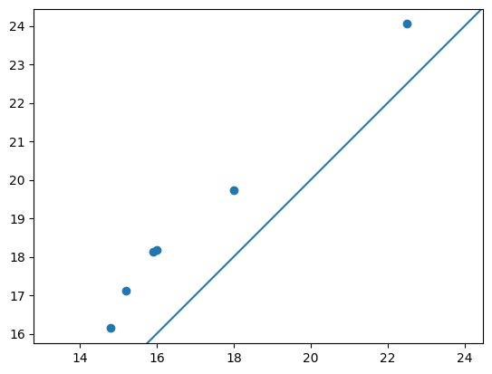
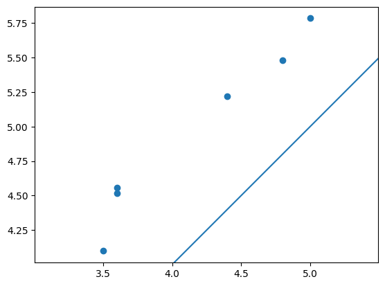
「インターフェースが違うだけで結果は同じ」なのか、実際に確かめてみます。ランダムな 600 bp テンプレート 5 本に対し、制約(プライマー長・Tm・GC・product size・塩/dNTP/DNA 濃度・返却数)を 3 実装で完全に揃えて design を回し、返ってきたプライマーペアを比較しました。環境は primer3 2.6.1、primer3-py 2.3.0、primer3-rs 0.1.0 です。
結果はきれいに揃いました。
- primer3 C 本体・primer3-py・primer3-rs の 3 実装が完全一致。5 テンプレート × 各 5 ペアすべてで、左右プライマー配列・product size・ペナルティ値(小数第 3 位まで)が完全に一致しました。
Rust バインディング ユースケース
primer3-rs が向いている場面
- 既存のツールチェインが Rust 製(
noodlesなどで BAM/VCF/FASTA を扱っている等)で、そこにプライマー設計を組み込みたい - 依存関係の少ない単一静的バイナリとして配布したい
- 大量配列を回すバッチで、コンパイル時の型安全性とパフォーマンスが欲しい
primer3-py で十分な場面
- 探索的な解析、インタラクティブな試行
- 既に Python 中心のパイプラインがある
C 本体を直接叩く場面
- シェルパイプラインに組み込むだけで十分
- サブプロセス起動で済ませたい
まとめ
- primer3 の新しい Rust バインディング primer3-rs が公開された。
primer3-sys/primer3/primer3-toolの 3 クレート構成 - API は primer3-py を踏襲しつつ、ビルダー + 型付き構造体 +
Resultで Rust らしく型安全 - C ソース同梱で導入は楽だが、ビルドに C コンパイラ + libclang が必要
- 既定値が primer3-py と一部異なるらしいので、移植時はパラメータに注意
primer3-py の資産をそのまま活かしつつ、Rust の型安全性とパフォーマンスを取り込みたい人にとって、有力な選択肢が増えたと言えそうです。
参考リンク
- primer3-rs(GitHub): https://github.com/fg-labs/primer3-rs
- primer3-rs(docs.rs): https://docs.rs/primer3/
- primer3-py: https://github.com/libnano/primer3-py
- primer3 本家 & マニュアル: https://primer3.org/