Shinyで96(384)-well plateのインターフェースを作ってみた

（以下の記事はR 3.6.3で試しています。）

Rはプロットに関する関数が充実して勘所をつかむと結構いろいろなお絵描きができます。例えば私は以前の記事でこんなアホなことをしています。

menseki.hatenablog.jp

そして、学生時代よく実験で使っていた96(384)-well plateもRで簡単に描けました。実際のコードは以下です。

wellplate <- expand.grid(x = 1:12, y = 1:8) # 96のとき
#wellplate <- expand.grid(x = 1:24, y = 1:16) # 384のとき
xlim <- range(wellplate$x) + c(-2, +2)
ylim <- rev(range(wellplate$y) + c(-2, +2))
plot(wellplate$x, wellplate$y, axes=FALSE, xlab=NA, ylab=NA,
     cex=3, asp=1, xlim = xlim, ylim = ylim)
rect(-1, -1, max(wellplate$x) + 1, max(wellplate$y) + 1)
text(x = 0, y = wellplate$y, LETTERS[wellplate$y])
text(x = wellplate$x, y = 0, as.character(wellplate$x))

96-well plate

96-well plateが描けるのならばこれをShinyのplotOutputに流して96(384)-well plateのインターフェースを作ってみようということで実際に作ってみました。以下のリンクから試すことができるようにしました。思い立ってすぐ突貫工事で作ったので現状バグが結構あると思いますのであしからず。気が向いたら修正していきます。

sabe.shinyapps.io

リンク先アプリ使用の様子（４倍速）

作ってみたはいいものの正直この程度のインターフェースのためにクライアントとサーバ間で何回も通信する設計になってしまっているのは実用的ではないと思っています（wellを選択するたびにその情報をサーバに送ってwell plateの全体図を再描画しています）。

まだjavascriptが書けないのでいつか書けるようになったらクライアン上でのみ処理するバージョンも書いてみたいです。

PythonでGGGenome検索

GGGenomeといえば配列を高速で検索してくれるサービスですが、そのトップページに記載の通り、REST APIの形でサービスを提供しているため、Pythonからも結構簡単に結果を取得できます。そこで、今回はpythonからGGGenome検索を行うためのスクリプトを描いてみました。

#!/usr/bin/env python3
import time
import requests

class GGGenome:
    # 前回アクセスした時間
    time_of_last_run = time.time()
    # アクセス間隔(秒間)
    dulation = 10

    # GGGenomeにクエリを投げ、結果をdictで返す
    def __call__(self, sequence, db="hg19", k=0, strand="both", nogap=False):

        if len(sequence) < 6:
            raise ValueError("query sequence should be 6 nt or more")
        self.sequence = sequence

        self.db = db
        
        if k * 4 > len(sequence):
            raise ValueError("number of mismatches/gaps should be 25% or less")
        self.k = k

        if strand == "both":
            self.strand = ""
        elif strand == "forward":
            self.strand = "+"
        elif strand == "reverse":
            self.strand = "-"
        else:
            ValueError("strand should be one of 'both', 'forward' or 'reverse'")

        if nogap:
            self.nogap = "nogap"
        else:
            self.nogap = ""

        # 前回のアクセスから最低{dulation}秒間待つようにする
        seconds_to_wait = GGGenome.dulation - (time.time() - GGGenome.time_of_last_run)
        time.sleep(max(0, seconds_to_wait))

        url = f"http://GGGenome.dbcls.jp/{self.db}/{self.k}/{self.strand}/{self.nogap}/{self.sequence}.json"

        result = requests.get(url)
        
        # アクセスした時間を更新する
        GGGenome.time_of_last_run = time.time()

        if result.status_code != 200:
            raise ValueError(f"HTTP Error. [status code: {result.status_code}]")

        if result.json()["error"] != "none":
            raise ValueError(f"searcher error. [{result.json()['error']}]")

        return result.json()

if __name__ == "__main__":

    import argparse
    parser = argparse.ArgumentParser(description="GGGenome command line")
    parser.add_argument('--db', type=str, default="hg19",
                        help="database name. default: hg19")
    parser.add_argument('-k', type=int, default=0,
                        help="number of mismachs allowed. default: 0")
    parser.add_argument('--strand', metavar='strand', type=str, default="both",
                        choices=["both", "forward", "reverse"],
                        help="which strand to query: default: both")
    parser.add_argument('--nogap', default=False, action="store_true",
                        help="whether or not to allow gap")
    parser.add_argument('sequence', metavar='sequence', type=str,
                        help="query sequence")
    args = parser.parse_args()

    gggenome = GGGenome()
    result_dict = gggenome(sequence=args.sequence, db=args.db, k=args.k, strand=args.strand, nogap=args.nogap)

    print(f"database: {result_dict['database']}")
    print(f"time: {result_dict['time']}")
    if args.strand == "both":
        print(f"    query(forward): {result_dict['summary'][0]['query']}")
        print(f"        number of hits: {result_dict['summary'][0]['count']}")
        print(f"    query(reverse): {result_dict['summary'][1]['query']}")
        print(f"        number of hits: {result_dict['summary'][1]['count']}")
    elif args.strand == "forward":
        print(f"    query(forward): {result_dict['summary'][0]['query']}")
        print(f"        number of hits: {result_dict['summary'][0]['count']}")
    elif args.strand == "reverse":
        print(f"    query(reverse): {result_dict['summary'][1]['query']}")
        print(f"        number of hits: {result_dict['summary'][1]['count']}")

スクリプトではGGGenomeクラスを定義しています。関数として実装しても良かったのですが、サーバに負荷をかけないように前回の検索から一定時間待機後次の検索をかける仕組みにしておきたかったのでクラス変数に前回のアクセス時刻とそこからの待機時間を記録できるようにしてあります。スクリプトを起動してから最初の検索までにも一定時間待機するため、bash等でスクリプトをループで回してもちゃんと一定時間待機すると思います。

本スクリプトのメインは以下です。

url = f"http://GGGenome.dbcls.jp/{self.db}/{self.k}/{self.strand}/{self.nogap}/{self.sequence}.json"

result = requests.get(url)

pythonのf-stringを用いてユーザーが指定したデータベース、ミスマッチ数、配列の向き、ギャップの許容、配列をもとにURLを構築し、requestsパッケージのget関数でHTTPリクエストをおこなっています。requestsのいいところの1つは結果をjson形式で受け取るとjsonメソッドで結果をPythonの辞書形式に直してくれるところだと思います。本スクリプトもこの機能を利用して結果を返しています。

参考

• GGGenome | ultrafast DNA search

二項分布とカイ二乗検定（と遺伝）

とある標本がとある分布に従ってサンプリングされたかを検定する方法として適合度の検定を行うことがあると思います。

今回は、得られた分離集団の形質の分離比が想定する遺伝様式に即しているかについての検定について見ていきたいと思います。

分離比に対する適合検定

例として、とある形質について、異なる表現型を示す純系2系統を用意し、F2を作成したとします。このとき表現型に分離が見られ、50個体中9個体が劣性（潜性）形質と思われる形質を示したとします。

この状況で、この形質は一遺伝子完全優性で説明されるか、つまり分離比は3:1であるかを調べるのに用いられるのが 乗検定だと思います。

とはいえこの現象は二項分布で自然に説明できる気がするのでまずは二項分布による検定を行ってみます。

二項分布で検定してみる

統計検定（両側）の流れは一般的に以下のようになると思います。

1. 帰無仮説 を立てる
2. 帰無仮説のもとデータが得られる確率 を求める
3. よりも起きにくい事象の確率の和 を求める（ 値）
4. があらかじめ設定した水準より低いかどうかを確認する

今回の例の場合、二項分布を用いると以下のような帰無仮説を設定できると思います。

観察された劣性（潜性）(と考えられる)形質を示す個体数は母数 の二項分布に従う

この仮定の上で、二項分布は以下のような確率分布を示します。

のときの尤度（帰無仮説のもとでの観察結果が得られる確率）を求めると

となります。また、これと同等またはより起きにくい事象の確率の和は図で言うところの赤とオレンジの部分の和であり、以下のようになります。

ということで帰無仮説は5%有意水準のもとで棄却できないことになります。 が増えてくにつれ計算が多くなって大変そうですが、Rを使えばbinom.test で実行できます。

> binom.test(x=9, n=50, p=1/4)

        Exact binomial test

data:  9 and 50
number of successes = 9, number of trials = 50, p-value = 0.3268
alternative hypothesis: true probability of success is not equal to 0.25
95 percent confidence interval:
 0.08576208 0.31436941
sample estimates:
probability of success 
                  0.18 

二項分布を正規分布で近似してみる

ところで、が十分大きいとき二項分布 は平均 、分散 の正規分布で近似できます。

そこで、二項分布から得られたとするデータを とすると は標準正規分布に従います。つまり標準正規分布表を用いて検定ができるのです。

また、標準正規分布から得られたデータを2乗すると 分布に従います。実際にを2乗してみると、

となり、ここで得られた式はまさに検定をする際に計算する と等価になっています。

まとめ

以上から、適合度検定は二項分布に従う確率変数が正規分布に従うと近似したときに検定として検定ができることがわかりました。カテゴリ数が3以上のときは多項分布に従うと仮定できると思いますので、多項分布による検定ができます。（RではEMTパッケージのmultinomial.testなどで実行できます。）ただ多くの場合は検定が使われているように思います。

参考

• https://en.wikipedia.org/wiki/Binomial_test
• https://en.wikipedia.org/wiki/Multinomial_test
• https://stats.stackexchange.com/questions/104468/understanding-the-chi-squared-test-and-the-chi-squared-distribution
• https://www.stat.berkeley.edu/~stark/SticiGui/Text/chiSquare.htm

Rust-BioでGzip圧縮されたFASTAを読み込む

Rustが注目を集めているらしいので流行りにのって使ってみました。

RustにはRust-Bioというバイオインフォマティクス用パッケージが存在します。そこで、今回はこれを用いてGzip圧縮されたFASTAファイルを読み込むプログラムを書いてみます。

まずはコードの全体から。

use structopt::StructOpt;
use std::fs::File;
use bio::io::fasta::{self, FastaRead};
use flate2::bufread::MultiGzDecoder;
use std::io::BufReader;
use std::ffi::OsStr;

#[derive(StructOpt)]
struct Opt {
    fasta: std::path::PathBuf,
}

fn main() {
    // コマンドライン引数をパース
    let args = Opt::from_args();

    // FASTAファイルを開く
    let file = File::open(&args.fasta).expect("Error during opening the file");

    // FASTAのリーダーを構築する(拡張子がgzの場合にMultiGzDecoderをはさむ)
    let mut reader: Box<dyn FastaRead> = match args.fasta.extension().and_then(OsStr::to_str) {
        Some("gz") => Box::new(fasta::Reader::new(MultiGzDecoder::new(BufReader::new(file)))),
        _ => Box::new(fasta::Reader::new(file)),
    };

    // FASTAのレコード毎にループ
    let mut record = fasta::Record::new();
    loop {
        reader.read(&mut record).unwrap();
        if record.is_empty() {
            break;
        }

        // 各レコードのIDと先頭10baseを表示
        println!("{} {}", record.id(), std::str::from_utf8(&record.seq()[0..10]).unwrap());
    }

}

使用するライブラリをスコープに持ち込む

use structopt::StructOpt;
use std::fs::File;
use bio::io::fasta::{self, FastaRead};
use flate2::bufread::MultiGzDecoder;
use std::io::BufReader;
use std::ffi::OsStr;

flate2::bufread::MultiGzDecoder は圧縮ファイルを解凍しつつ読み込むために使います。 flate2にはGzDecoderも存在しますがこれはhtslibのbgzipコマンドのようなBGZF ブロックに分けて圧縮するようなタイプのファイルに対応していないようです。

もう一つ重要なのはbio::io::fastaです。このモジュールが提供するReaderにより FASTAを適切にパースすることができるようになります。

FASTAリーダーを構築する

// FASTAのリーダーを構築する(拡張子がgzの場合にMultiGzDecoderをはさむ)
let mut reader: Box<dyn FastaRead> = match args.fasta.extension().and_then(OsStr::to_str) {
    Some("gz") => Box::new(fasta::Reader::new(MultiGzDecoder::new(BufReader::new(file)))),
    _ => Box::new(fasta::Reader::new(file)),
};

圧縮されていないFASTAをパースするときはfasta::Reader::new(file)、 gzip圧縮されているFASTAをパースするときはfasta::Reader::new(MultiGzDecoder::new(BufReader::new(file))) を用います。それぞれ場合分けしてコードを書くと冗長になるためここではBoxに入れて 1つの変数に格納できるようにしています。このとき変数の型としてFastaReadトレイトを指定することで、 FastaReadトレイトを実装するオブジェクトを格納することができるようにしています。

Rustは型に厳しいようなのでこの辺がなれるまで大変だと個人的には思いました。

レコードを1つずつ読み込む

// FASTAのレコード毎にループ
let mut record = fasta::Record::new();
loop {
    reader.read(&mut record).unwrap();
    if record.is_empty() {
        break;
    }

    // 各レコードのIDと先頭10baseを表示
    println!("{} {}", record.id(), std::str::from_utf8(&record.seq()[0..10]).unwrap());
}

fasta::Readerオブジェクトにはrecordsメソッドがあるのですが、先ほどのようなBoxでラップする様な方式をとると使えなくなるみたいなので、readメソッドをループ毎に呼び出し、レコードを1つずつ読み込みます。

最後までレコードを読み込むと、Recordオブジェクトのis_emptyメソッドがtrueを返すようになるのでループを抜け出すようにします。

RecordオブジェクトにはidメソッドによってIDに、seqメソッドによって配列にアクセスできます。他にもいくつかのメソッドがありますのでドキュメントを参照してみてください。

以上がGzip圧縮されたFASTAファイルを読み込む（非圧縮ファイルも受け付ける）プログラム解説でした。

Python等と異なりコンパイルを通すまでが一苦労ですが、安全で速い言語ということなので、選択肢の一つとしていきたいと思いました。

枝豆データセットを分類してみた

この間会社の先輩から「IT農家のラズパイ製ディープ・ラーニング・カメラ」（2020、小池誠）という本を貸していただいたので読んでみました。その中でディープラーニングの応用例として枝豆の莢の画像を2粒莢と3粒莢に分けるというタスクが紹介されていました。このデータセットについては親切にGitHub上に公開されています。今回はこれをディープラーニングではない方法で分類できないか実験してみました。

使用言語はPythonで以下のモジュール・関数群をインポートしています。

このインポートの様子からもわかるように今回はランダムフォレストでの分類を試みます。

import numpy as np
import pandas as pd
import matplotlib.pyplot as plt
from skimage.measure import label, regionprops
from skimage.filters import threshold_otsu
from skimage.morphology import opening, square
from sklearn.ensemble import RandomForestClassifier
from sklearn import metrics

データダウンロード・整形

まずはデータセットをGitHubからダウンロードして整形するところからです。

以下のようにして、GitHubにあるスクリプトを参考に多少Numpy配列のShapeを変更してデータセットを構築します。

このデータセットはすでに学習用と評価用に分けられているのでそれをそのまま用います。

#ダウンロード
!wget "https://github.com/workpiles/soybeans_sorter/raw/master/soybeans_gray.npz" -O soybeans_dataset.npz -q

#ダウンロードしたデータセットの読み込み
IMAGE_HEIGHT = 48
IMAGE_WIDTH = 64

def load_data():
    data = np.load("soybeans_dataset.npz")
    x_train = data['x_train'].astype('float32') / 255.
    x_test  = data['x_test'].astype('float32') / 255.
    x_train = x_train.reshape([-1, IMAGE_HEIGHT, IMAGE_WIDTH])
    x_test  = x_test.reshape([-1, IMAGE_HEIGHT, IMAGE_WIDTH])
    y_train = data['y_train']
    y_test  = data['y_test']
    return x_train, y_train, x_test, y_test

X_train, y_train, X_test, y_test = load_data()
print(X_train.shape, y_train.shape, X_test.shape, y_test.shape)

#画像の確認（学習用データの先頭10個の画像を表示）
#fig, ax = plt.subplots(1, 10, figsize=(12, 6))
#for i in range(10):
#    ax[i].imshow(X_train[i], cmap="gray")
#    ax[i].axis('off')
#    ax[i].set_title("label:%d"%(y_train[i]))
#plt.show()

(600, 48, 64) (600,) (580, 48, 64) (580,)

特徴量抽出

ディープラーニングでは画像と教師データを入力すると自動で特徴量の抽出を学習してくれますが、今回はそれを用いないので自分で特徴量を抽出する必要があります。

個人的に形を見れば分類できそうに感じたので形に関連する特徴量を画像から抽出するコードを書いていきます。

まずは画像における枝豆の領域をマスク画像として抽出したいので大津法による閾値の計算を行い、画像を2値化します。

example_image = X_train[0]
thre = threshold_otsu(example_image)
mask = opening(example_image < thre, square(3)) # opening関数で細かいノイズを除去して境界をなめらかにしています
fig, ax = plt.subplots(1, 2, figsize=(6, 4))
ax[0].imshow(example_image, cmap="gray")
ax[0].set_title("raw image")
ax[1].imshow(mask, cmap="gray")
ax[1].set_title("binary image")
plt.show()

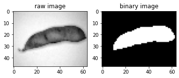
枝豆のマスク画像を作成できたので、 skimage.measure の regionprops 関数でマスク画像に含まれる連続した白い部分ごとに抽出することができる各種特徴量について計算します。

regions = regionprops(label_image=label(mask))
# マスク画像の中には小さなノイズが含まれるので、最も面積が大きい領域から得られる特徴量を採用する
prop = sorted(regions, key=lambda x:x.area, reverse=True)[0]

上記コードによって prop という変数に計算された特徴量が格納されます。

形を定量する特徴量としてHu momentsというものがあるのでこれを用います。これは図形が回転したり拡大縮小しても変化しない特徴量で形を数値化していると考えることができると思います。Hu momentsは一般に7次元のベクトルとして表されます。

また、画像取得時のカメラと対象の距離が固定されているとのことなので、枝豆の面積や長さ等の特徴量も利用できるのではと思ったのでこれらも含めたいと思います（本では2粒莢と3粒莢で長さが等しいものもあると紹介されていますが）。

# 利用する特徴量の名前
feature_names = [
    "hu moments 1",
    "hu moments 2",
    "hu moments 3",
    "hu moments 4",
    "hu moments 5",
    "hu moments 6",
    "hu moments 7",
    "perimeter", # 周長
    "area", # 面積
    "major axis length", # 楕円近似したときの長い方の長さ？
    "eccentricity", # 偏心率　細長さの度合い？
]

print(f"hu moments: {prop.moments_hu}")
print(f"perimeter: {prop.perimeter}")
print(f"area: {prop.area}")
print(f"major axis length: {prop.major_axis_length}")
print(f"eccentricity: {prop.eccentricity}")

hu moments: [ 3.39570803e-01  8.53334557e-02  2.62741796e-03  4.25716946e-04
  1.16743483e-07 -1.29062051e-05 -4.34843423e-07]
perimeter: 127.25483399593904
area: 647
major axis length: 57.180643020830146
eccentricity: 0.9617073387929369

これらの特徴量を抽出しnumpyのベクトルとして返す関数を用意します

def extract_features(img):
    thre = threshold_otsu(img)
    mask = opening(img < thre, square(3))
    regions = regionprops(label_image=label(mask), intensity_image=img)
    prop = sorted(regions, key=lambda x:x.area, reverse=True)[0]
    features = np.concatenate((prop.moments_hu, [prop.perimeter, prop.area, prop.major_axis_length, prop.eccentricity]))
    return features

この関数を用いて X_train および X_test からデータ数*特徴量数の行列（ new_X_train 、 new_X_test ）を作成します。

new_X_train = np.array([extract_features(x) for x in X_train])
new_X_test = np.array([extract_features(x) for x in X_test])
# shapeの確認
print(new_X_train.shape)
print(new_X_test.shape)

(600, 11)
(580, 11)

ランダムフォレストによる学習

それではいよいよランダムフォレストによる学習を実行します。今回は木の数を200に設定しました。

forest = RandomForestClassifier(n_estimators=200, random_state=0)
forest.fit(new_X_train, y_train)
y_pred = forest.predict(new_X_test)
print(f"accuracy: {metrics.accuracy_score(y_test, y_pred)}, F1: {metrics.f1_score(y_test, y_pred)}")

accuracy: 0.9913793103448276, F1: 0.9914236706689538

無事正答率、F値ともに0.99の精度で評価用データセットを分類することができました。

各特徴量の重要度

ランダムフォレストの良い点として各特徴量の予測に対する重要度を計算することができます。そこでここでも重要度を算出してプロットしてみます。

importances = forest.feature_importances_
std = np.std([tree.feature_importances_ for tree in forest.estimators_], axis=0)
forest_importances = pd.Series(importances, index=feature_names)

fig, ax = plt.subplots(figsize=(6, 4))
forest_importances.plot.bar(yerr=std, ax=ax)
ax.set_title("Feature importances using MDI")
ax.set_ylabel("Mean decrease in impurity")
fig.tight_layout()

print(forest_importances)

hu moments 1         0.131664
hu moments 2         0.215949
hu moments 3         0.021450
hu moments 4         0.031299
hu moments 5         0.006485
hu moments 6         0.039046
hu moments 7         0.009430
perimeter            0.102604
area                 0.051952
major axis length    0.206005
eccentricity         0.184116
dtype: float64

Hu momentsの2つ目とeccentricityが重要だということがわかったので、この2つをx軸、y軸にとり学習用データセットをプロットしてみます。

赤はつまり3粒莢、青は2粒莢を表しています

plt.figure(figsize=(6, 4))
plt.scatter(new_X_train[np.where(y_train == 1.0), 1], new_X_train[np.where(y_train == 1.0), 9], c="red")
plt.scatter(new_X_train[np.where(y_train == 0.0), 1], new_X_train[np.where(y_train == 0.0), 9], c="blue")
plt.xlabel(feature_names[1])
plt.ylabel(feature_names[9])
plt.show()

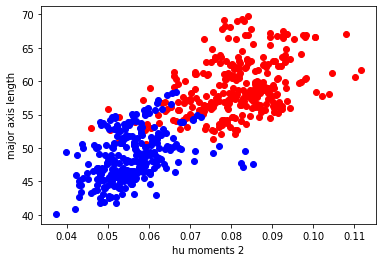
確かに、2つの特徴量だけでも結構うまく分離できそうなことがわかります。

まとめ

今回は「野菜を自動仕分けするAIマシン製作奮闘記 IT農家のラズパイ製ディープ・ラーニング・カメラ」にて紹介されている枝豆2粒莢・3粒莢分類タスクをランダムフォレストフォレストで分類することを考えてみました。

ランダムフォレストなど、ディープラーニング以外の機械学習手法を画像分類に適用する場合、最初に画像からいくつかの特徴量を抽出する必要がありました。今回のタスクと入力画像は比較的単純であり背景が統一されていてきれいだったために簡単に特徴量を抽出することができ、結果的にランダムフォレストでの分類ができました。

また、ランダムフォレストなどの手法はディープラーニングに比べ計算コストが低いためCPUでの計算が簡単にできます。

実際の現場では両者の特性を理解し適材適所で活用していくのが重要だと感じました。

参考

CQ文庫シリーズ 野菜を自動仕分けするAIマシン製作奮闘記 IT農家のラズパイ製ディープ・ラーニング・カメラ 小池誠 著 2020 CQ出版株式会社

GitHub - workpiles/soybeans_sorter: 枝豆選別の実験

ラズパイで植物の定点観測

数年前にRaspberry Piを購入してたのですがちょっと遊んだまま放置になっていたので何か意味のある 装置を作ってみようと最近になって思い立ったので作ってみました。

作ったものはセルトレー上で育てている植物を上からカメラで定点観測するというものです。

用意したもの

• Raspberry Pi 3 model B+
• Raspberry Pi Camera V2
• ブレッドボード
• LED
• ジャンプワイヤー
• 三脚
• 土台となる板
• など…

正直定点観測だけならLEDやブレッドボードはいらないのですが、同時にGPIOについても勉強しようと思い用意しています。

組み立て

ハードの部分の組み立てについては以下の写真に示すような構造にしました。

要はカメラの三脚に土台となる板を取り付け、その上にカメラモジュールを接続したラズパイ、その他周辺機器を接続した感じです。

Raspberry Piとカメラモジュールをいい感じにセルトレーの直上に設置した様子

日曜大工したことない私が何も見ないで作ったので結構適当な設計になっていますが形にはなっているのでよしとします。

LEDはGPIO4番端子に取り付け、プログラミングで制御できるようにしています。（もちろん抵抗はつけています。）

写真をとるスクリプト

続いてソフトの方を開発していきます。やったことはカメラモジュールを操作して写真を撮影するスクリプトの作成です。以下のようなスクリプトを書きました。

#!/usr/bin/env python3 
import picamera
import RPi.GPIO as GPIO
import time
import os.path as path

# properties for image
PICTURE_WIDTH = 800
PICTURE_HEIGHT = 600
FRAMERATE = 15

# directory to save image
SAVEDIR = path.join("/", "home", "pi", "plant_observation", time.strftime("%Y%m%d"))

# GPIO setup
GPIO.setmode(GPIO.BCM)
GPIO.setup(4, GPIO.OUT)

# blink LED for indicate taking a picture
for i in range(5):
    GPIO.output(4, GPIO.LOW)
    time.sleep(0.5)
    GPIO.output(4, GPIO.HIGH)
    time.sleep(0.5)

# take a picture
cam = picamera.PiCamera()

cam.resolution = (PICTURE_WIDTH, PICTURE_HEIGHT)
cam.framerate = FRAMERATE

filename = time.strftime("%Y%m%d%H%M%S") + ".jpg"

save_file = path.join(SAVEDIR, filename)

cam.start_preview()
time.sleep(5)
cam.capture(save_file)
cam.stop_preview()

# LED off
GPIO.output(4, GPIO.LOW)
GPIO.cleanup()

上記スクリプトは /home/pi/plant_observation/ という名前のディレクトリに hourly_camera.py という名前で保存しました。

カメラはルート権限でないと動かせないようなので上記スクリプトはルート権限で実行しました。

定期的に写真を撮るための設定

Linuxにはcronという仕組みがあり、それにより定期的にコマンドを実行できるので、この仕組みを用いて、自動的に設定した時間に写真が撮られるようにします。

ルートユーザでcronコマンドを打ちます。

crontab -e

するとテキスト編集画面にになるので、最終行に以下の一行を追加します。

00 * * * * cd /home/pi/plant_observation/ ; python3 hourly_camera.py >>log 2>&1

この行の意味は毎時00分に先ほど作成したスクリプトを実行するという意味になります。

以上で植物の簡易的な植物定点観測システムができあがりました。

時間があればさらに環境情報（気温、湿度等）の記録などの機能を付け加えて、 より有意義なシステムにアップグレードしていきたいと思っています。

ちなみに取れた写真はこんな感じです。（ちょっとピントが合ってない感じがあったのでこの後カメラのレンズ部分を回転させて調整しました。）

今回の装置で取れた写真

ImageJで葉面積を測ってみた

ImageJを使って単純な方法で画像から葉面積を測ってみました。大まかな方法としては、画像から緑の部分を選択して選択された部分の面積（ピクセル数）を数える感じです。

RGBからLab色空間に変換する

RGBのGチャンネルが高いピクセルが緑だと思いそうですが案外そうでもありません。Lab色空間にすることでa*の座標軸の小さい方が緑になっているので、まずはRGBからLabに変換します。

ImageメニューのTypeからLab Stackを選択します。変換には多少時間がかかるようです。

RGBからLabに変換

変換が終わると以下のように画像がグレースケールに代わり、さらに画像の下にスクロールバーが現れます。

Labに変換し終わった図

スクロールバーを真ん中に移すことでa*軸の値のグレースケールを表示できます。

以下のように、画像の左上に 2/3 (a*) という表記がされていればOKです。

a*座標のデータを表示

Thresholdを設定する

続いてImageメニューのThresholdを選択肢、バックグラウンドと葉っぱを区別するための閾値を設定します。

Thresholdを設定

Thresholdを選択すると以下の図のように小さなウィンドウが表示されパラメータを設定できます。パラメータを適宜設定して、葉っぱの部分が赤く選択されるようにします。もし、Dark backgroundにチェックがついていたら外します。

葉っぱの部分を選択した図

面積を計算する

次にいよいよ面積を計算するための設定に入ります。AnalyzeメニューのSet Measurements...を選択します。

Set Measurements...の選択

すると以下のようなウィンドウが現れるのでAreaを選択し、Limit to thresholdにチェックをつけます。これをすることで現在設定しているThresholdで選択されている部分の面積を測ってくれます。

Set Measurements...の設定項目

Set Measurements...のウィンドウでOKを押したら、AnalayzeメニューのMeasureを選択します。

Measureを選択

以下のようなウィンドウが現れて面積がピクセル数で表示されました。

葉面積計測結果

ちなみに先ほど説明したLimit to thresholdのチェックを外してMeasureを再度選択すると画像全体の面積がでます。これらの値の比をとることで被度的なものが得られるかもしれません。

画像全体の面積計測結果

今回の方法はかなり単純なので葉が緑でない部分があったり、逆に地面に葉とは関係ない緑色の部分があったりするとその部分が計算に含まれなかったり含まれたりするので厳密性をあげるならもう少し工夫が必要かもしれません。